The Simulation of Simplicity: Give a boost to your code
1. “A mathematician is a device for turning coffee into theorems.”
Alfréd Rényi
In the 1980s, a famous illusionist made the Statue of Liberty disappear in front of a stunned crowd. Mathematicians also have this talent of making things disappear, and on top of that, they do not hide their secret. This is what happened in 1990 when two mathemagicians, Herbert Edelsbrunner and Ernst Peter Mücke, published an article titled "Simulation of simplicity: a technique to cope with degenerate cases in geometric algorithms” [1]. This paper, now cited more than eleven hundred times, revealed a beautiful method designed to remove one of the sometimes-painful aspects of computational geometry: the degenerated cases. This method has since become a standard tool for scientific computing engineers, used particularly in geometrical algorithms at the heart of the modeling of the geological structures. In this blog post, with a minimum of math (only determinants needing to be known) I will try to explain the essence of the Simulation of the Simplicity.
2. “There are some things so serious you have to laugh at them.”
Niels Bohr
Put simply, degenerated cases in geometric algorithms are situations where the geometric objects being manipulated are not in general positions. For example, when thinking of two points in space, one would first think of two distinct points in space. This is the generic situation. If the two points coincide, it is a special case. Similarly, when thinking of three points on a plane, one would first visualize a triangle, the generic case. The cases where the three points are aligned or coincident are particular cases. Geometric degeneracies are not problematic in themselves because after all, in a world without corner cases, we would be going around in circles... But as pointed out by the authors: "when it comes to implementing geometric algorithms, degenerate cases are very costly, in particular, if there are many such cases that have to be distinguished" [1]. Indeed, to ensure the robustness of a geometry code, it is necessary to identify all the corner cases and to ensure that the program handles each of them properly. This work, which can be tedious, has consequences on the length, complexity, and might “obscure the centrality of the non-degenerate cases” [10].
3. “You enter a completely new world where things aren't at all what you're used to.”
Edward Witten
Such was my feeling upon first reading the article we are discussing here, as the promise of the method seemed astonishing to me. Because what the authors propose is just to make special cases disappear. This what simulating simplicity means: simulating a world without corner cases. We will see that with a wave of "magic perturbations" we will make the problem disappear. But before we reach this wonder, we must first focus on the structure of geometry programs.
4. “The truth always turns out to be simpler than you thought.” Richard P. Feynman
A geometry program can be schematically considered as a set of processing units that perform calculations and "switches", called predicates, which guide the program in one branch or another. By definition, a predicate is a function that returns true or false, but in practice predicates return +1 for true, -1 for false, and 0 for degenerate cases. Now, here is the excellent news of this section: some predicates, among the most used, are built using matrix determinants that become zero when the data is degenerate. More specifically, these predicates calculate the sign of a determinant and return +1 if it is positive, -1 if it is negative, and 0 when the determinant vanishes indicating a degenerate case.
To make things more concrete, here are two commonly used examples.:
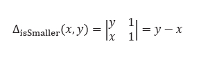
- IsSmaller: it takes as input two real numbers x and y and returns +1 if x is smaller than y, -1 if x is greater than y, and 0 if x and y are equal (degenerated case). The determinant associated with this predicate is:
- Orientation2D: let us consider three points A, B, C in the plane and the determinant below:
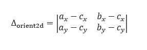
One can prove that the sign of this determinant is strictly positive if the points A, B, C are arranged in counterclockwise order, and strictly negative if the points are in clockwise order. If the points are collinear or coincident, the determinant is equal to zero (degenerated case).
At this stage, you can legitimately wonder why the existence of predicates expressed by determinants is good news. Well, imagine a world where these determinants never cancel out. In this world, we would never encounter specific cases! It turns out that this world exists, it was created by mathematicians in the 20th century...
5. “Young man, in mathematics you don't understand things. You just get used to them.”
John von Neumann
As we will detail in the next section, SoS embeds and perturbs the coordinates of geometric objects in a set larger than real numbers called the set of the hyperreals. It is in this somewhat strange set that degenerate cases will disappear. In the following, I will briefly present the concepts necessary for understanding the method while avoiding theoretical difficulties. The set of hyperreals is an ordered set that contains real numbers as well as other elements called infinitesimals. Although an infinitesimal can be positive or negative, it does not have a numerical value. In fact, if it is strictly positive, then it is smaller than any strictly positive real number. It is an indeterminate "infinitely small" as we could say.
As mathematicians like to do calculations, they have defined the usual operations and a set of rules on the hyperreals. Those mentioned below will be useful to us later. We note ε an infinitesimal in all that follows.
- One can multiply or divide an infinitesimal by any real number.
- One can multiply infinitesimals.
- All positive second-order infinitesimals are smaller than the any positive first-order infinitesimal. For example:
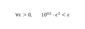
And you could replace 1052 with an arbitrary larger number!
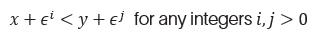
- One consequence is that:

- If x and y are two real numbers such as x<y,
6. “The whole is more than the sum of its parts.”
Aristotle
It is now time to assemble the different elements obtained so far. Let us recall the question we want to answer: how can we ensure that the determinants defining our predicates never cancel out? The answer provided by Edelsbrunner and Mücke is this: add perturbations constructed using infinitesimals to the input data. These perturbations, which depend on the problem at hand, are called symbolic (or virtual) because they are never really applied to the data. Let’s take an example that will help better understand the idea.
Let’s imagine we work out an algorithm taking only two points in the plane A(ax,ay) and B (bx,by), and depending only on the following predicate:

We define the perturbation as follows:

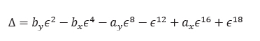
It is now necessary to verify that the determinant computed on the perturbed coordinates never cancels out. The property of multilinearity of determinants allows us to write:
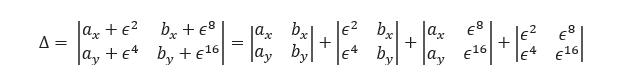
Or after ordering the terms in increasing order of the powers of ϵ :
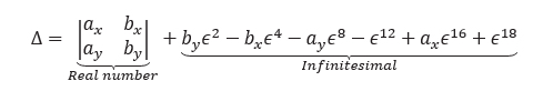
The structure of the determinant above is particular: the first term is the determinant of the unperturbed data. This is a real number, positive, negative, or zero. All the other terms being infinitesimals, their sum is an infinitesimal.
Let’s see what happens if we run the program on data in a generic situation. In this case,
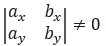
and the sign of this determinant gives the sign of Δ. This is very important! this means that the introduction of the perturbations has not introduced degenerate cases. I will say it differently: if the points are in a generic situation, the perturbed version coincides with it.
Now, what if the points are in a particular configuration? Then we have
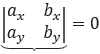
and
Using the rules of calculation with infinitesimals, the sign of Δ is given by the sign of the first non-zero coefficient of an infinitesimal ϵí . If by≠0, then the sign of by gives the sign of Δ, otherwise we consider bx etc… Let’s see the worst-case scenario when all the coordinates collapse to zero (A=B=O). We have then:
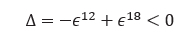
Meaning the points are seen in generic configuration oriented clockwise!
7. “This isn't right. This isn't even wrong.”
Wolfgang Pauli
Perhaps this is what you are thinking? Indeed, a computer does not handle all real numbers, but only a finite subset called the floating-point set. Therefore, substituting floating point arithmetic for the assumed real arithmetic will highly likely result in numerical errors. In particular, the result of a theoretically zero determinant may not be zero in floating point arithmetic. Similarly, a theoretically positive determinant may be evaluated as negative in floating point arithmetic. In short, the method seems unapplicable unless exact calculations can be performed on a computer. If you are a regular reader of the blog posts, this will not concern you further as you already know this is possible. Of course, this comes with a numerical cost and thus impacts the execution time of the code, although it can be optimized with specific techniques. But that's another story...
Another issue related to the method is that the result obtained on perturbed data may show "geometrical defects" such as geometric objects with zero areas or volumes. To illustrate this, imagine that in the example presented in the previous section, we create a triangle each time the points O, A, B are clockwise oriented. Since SoS transforms the colinear cases into clockwise cases, we might create flat triangles…Depending on the problem being addressed, it may be desirable to remove these defects. In practice, those who choose to apply SoS have therefore deemed that the cost of post-processing is preferable to managing all the possible corner cases.
7. “Out of clutter find simplicity.”
Albert Einstein
"The main goal of this paper is to argue against the belief that perturbation is a “theoretical paradise”” can be read in [3]. It is mainly the difficulties exposed previously that have led the authors of this article, remarkable in other respects, to this observation. And yet, since its publication, the method SoS has found its way into multiple complex applications such as [4][5][6][7][8][9][11] ... The list seems endless. It confirms the intuition of Edelsbrunner and Mücke when they wrote: “the authors believe that SOS will become a standard tool for implementing geometric algorithms” [1]. But this method has something more to me, a particular charm: perhaps it is because by invoking elusive little nothings, SoS reveals to us their power to transform the world.
Bibliography
[1] Edelsbrunner, H., & Mücke, E. P. (1990). Simulation of simplicity: a technique to cope with degenerate cases in geometric algorithms. ACM Transactions on Graphics (tog), 9(1), 66-104.
[2] Shewchuk, J. R. (1999). Lecture notes on geometric robustness. Eleventh International Meshing Roundtable, 115-126.
[3] Burnikel, C., Mehlhorn, K., & Schirra, S. (1994, January). On degeneracy in geometric computations. In Proceedings of the fifth annual ACM-SIAM Symposium on Discrete algorithms (pp. 16-23).
[4] Aftosmis, M. J., Berger, M. J., & Melton, J. E. (1998). Robust and efficient Cartesian mesh generation for component-based geometry. AIAA journal, 36(6), 952-960.
[5] Lévy, B. (2016). Robustness and efficiency of geometric programs: The Predicate Construction Kit (PCK). Computer-Aided Design, 72, 3-12.
[6] De Magalhães, S. V. G. (2017). Exact and parallel intersection of 3D triangular meshes. Rensselaer Polytechnic Institute.
[7] Cabiddu, D., Attene, M. (2017). ϵ-maps: Characterizing, detecting and thickening thin features in geometric models. Computers & Graphics, 66, 143-153.
[8] Meng, Q., Wang, H., Xu, W., & Zhang, Q. (2018). A coupling method incorporating digital image processing and discrete element method for modeling of geomaterials. Engineering Computations, 35(1), 411-431.
[9] Diazzi, L., Panozzo, D., Vaxman, A., & Attene, M. (2023). Constrained Delaunay Tetrahedrization: A Robust and Practical Approach. ACM Transactions on Graphics (TOG), 42(6), 1-15.
[10] Yap, C. K. (1990). Symbolic treatment of geometric degeneracies. Journal of Symbolic Computation, 10(3-4), 349-370.
[11] Lévy, B. (2024). Exact predicates, exact constructions and combinatorics for mesh CSG. arXiv preprint arXiv:2405.12949.
